CISM c1311 course: Differential geometric methods for multi-body-system simulations (part 2)
(Part two of a series on a seminar I attended at the International Center for Mechanical Sciences; part one is here.)
After the brief intro to Lie groups, we were shown applications of Lie group theoretic integrators to various problems in mechanics. It's easy to see how the theory applies to rigid bodies. The movements of a rigid body are just translations and rotations, and these are easily represented by a Lie group often referred to as SE(3), the semidirect product of SO(3) and R(3)."Semidirect product" refers to how elements in SE(3) combine, once given combination laws for its component groups. There's some ambiguity in the literature, actually, as some people call the direct product of R(3) and SO(3) (denoted R(3)xSO(3)) by the name SE(3).
The difference is, in a direct product elements from different group components do not mix. Example, suppose you have two elements in R(3)xSO(3), let them be (t1, R1) and (t2, R2). Then, the composite of the two elements is simply (t1+t2, R1*R2). Each component of the direct product uses its own combination law.
Flexible bodies, which can deform in motion, seem to pose a challenge to a Lie group based formalism, but that is not so. They're usually modelled by using a few coordinate frames to represent various "parts" in them, and these frames can move relative to each other the same way rigid bodies do. Of course, you'd have some kind of stress calculations to see how applying forces/torques to the object twists these frames relative to each other. In any case, an extension of the Lie group theory to flexible bodies moving 'freely' is trivial.

"Constraints" are more interesting. These are hard conditions imposed on the evolution of a physical system; an example might be, never go inside the floor (no ghosting!), or to revolve around a hinge joint, or keep at a fixed distance from some point. Just like rigid bodies, which are just simplifications and do not actually exist, constraints are also, in some sense, non-physical. When two objects collide, they will deform, slightly. The length of a pendulum varies. A hinge changes shape, even if slightly. No position constraint is absolutely enforced, in nature. Still, rather than worry about how nature goes about almost enforcing a constraint (which adds more degrees of freedom, elasticities and dampings you need to tune, and so on), all to model motions that are on the order of micrometers, engineers prefer to say, the position constraint is enforced.

Usually one distinguishes unilateral constraints (don't go inside a region) from 'proper' constraints like the hinge joint, and for now I'll talk about the second kind. It can be represented, mathematically, by some function, which takes the current system state and should return 0 if the constraint is satisfied.
Typically a system state has position and velocity variables. A large class of constraints, often called "holonomic" constraints, only require position. That means, the function you need to specify them only needs the position as an argument; as a consequence, these constraints put a hard limit on where the system can be, what states it can reach. They define a subspace, which you can think of as some shape inside the space of possible states. For example, a 2D pendulum with the mass constrained to be at a fixed length away from a pivot must be somewhere on a circle.

They can be rewritten as constraints on velocity (or acceleration) too. As an example, consider the pendulum in 2D again. The velocity the pendulum mass can have is always perpendicular to the pendulum arm; a component of velocity along the pendulum arm means the distance to the pivot would change. In general, since holonomic constraints define a "shape", you can always see which directions of motion (starting from some point) keep you on the shape and which will take you away.
There are also "non-holonomic constraints", which constrain the velocities a system can have, but not necessarily where it can eventually arrive at. An example is provided by rotations, again. Suppose I am allowed to rotate the GIMP monkey head only along the world X and world Y axis. Even so, there's a sequence of rotations along these two axis which has the same effect to a world Z rotation (example: world-X 90 degrees, then world-Y 90 degrees, then world-X -90 degrees, is the same as world-Z 90 degrees). Even if I'm not allowed to apply a Z rotation, I can still get there.
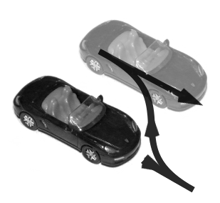
Another example is parallel parking. Usually, cars don't slide sideways. However, with a combination of steering and moving in the direction the front wheels point, I could take a car side-ways relative to its starting position.
This is connected to the Lie algebra again, and to an operation called the Lie bracket, which takes two vectors in the Lie algebra as argument (order matters!) and returns a third. If the equation is "[A, B] = AB - BA = C" its meaning, (very) roughly speaking, is the following: if you went for a 'very short' step in direction A, then a 'very short' step in direction B, then a 'very short' step in the reverse direction of A, and a 'very short' step in the reverse direction of B, then you'd end up at a point which is in direction C from where you started.
The Lie bracket is therefore quite important in control theory. In some fairly mild conditions, it tells you whether a certain collection of actuators is, in principle, capable of taking your systems to some target state. In some more stringent conditions, it might even tell you how to get there, meaning, how to use the actuators to get where you want.
Non-holonomic constraints are fairly weird though and we didn't insist a lot on them. They mostly are encountered with vehicles, where "no side slipping" is often assumed of the wheels. Important, therefore, if you want to create a driving algorithm for a car. If you want to simulate that car operating on slippery roads however, then you don't need to bother with them. Holonomic constraints are weird enough.
(Actually, momentum conservation is also a non-holonomic constraint, but for this particular constraint, Lie group integrators are very well suited. This will be covered in another post.)
One problem is that there are more ways for them to enter into the equations. You could use a constraint function on positions, or its version that operates on velocities, or even its acceleration version. All choices are valid; each has its problems.
It comes down to, what is easy to do, for some given application (physical system model). If you enforce the constraint on positions, then the system will stay inside the subspace which contains the allowed positions, but its velocity and acceleration may behave weirdly and must be stabilized somehow. If you constrain on velocities, then they will be ok, but even so the system will drift away from the allowed subspace because of numerical error, and must be brought back ('projected back' to the allowed subspace).
It's difficult to decide, from the seminar, which version is better. Some of the lecturers preferred to use constrained positions. Some preferred the constrained accelerations. The difference between the approaches is the 'index' of the differential-algebraic equations (DAEs) being solved.

The way one adds constraints to a dynamic model is via some kind of 'Lagrange multipliers' (the λ in the equations). It's a fancy term, but what it means is pretty simple: they are the forces that fight back if you try to move in a forbidden direction. To take the pendulum example again, you can imagine the pendulum moving under the influence of gravity and a constraint force that acts through the pendulum arm.
The simple integrators for non-constrained systems would compute the forces acting on the system in the current state, so as to get the accelerations, and then run an integration scheme on that. When there also constraints, the constraint forces (Lagrange multipliers) also must be computed, often from some algebraic equations, obtained from the constraint function. The "index" of the DAE is the number of times you need to differentiate the constraint equations to get the first time derivative of the constraint forces. So, for example, if the constraint equation is on acceleration, the index is 1 (because you need to differentiate it once to get the time derivative of the Lagrange multipliers). If the constraint is on position, the index is 3; the constraint must be derived twice to bring it to acceleration form, then once more to get the Lagrange multiplier derivative.
In theory, if you have equations for the system's acceleration and the time derivatives of the Lagrange multipliers, the problem becomes expressible as an ordinary differential equation (ODE) for which simple integrators suffice. In practice, you need to make sure the constraints hold; an integrator would otherwise drift to nonsense solutions because of numerical error.
So one option is to use the constraint on acceleration (DAE index 1) to get the Lagrange multipliers, do an integration step, and once in a while ensure the positions and velocities are obeying the constraints by reprojecting them to the allowed shape. It's often said that index 1 equations are friendlier to solve, as you don't run in numerical troubles, even if you have the extra complexities of reprojections.
Another option that one lecturer (Carlo Bottasso) argued for is to use the index 3 version. The basic outline here is, you make a first "guess" about what the multipliers should be, run the integrator, and see how far away you are from respecting the position constraint. You adjust your guess to make this error smaller by some optimization procedure (typically Newton-Rhapson). You are guaranteed to enforce the position constraint this way, and you rarely need to reproject velocities and accelerations, so there should be less computational load ...
But there's a problem. It turns out that if you make your simulation time step too small, the accuracy of the method suffers. This is bad; and counterintuitive. The finer the discretization, the better the approximation should be, right?
Not in a naive DAE index 3 solver though. What happens is that, because of numerical error, there will be some deviation between where your optimization should go for its next guess, and where it actually goes. This error turns out to depend on negative powers of the timestep, so the smaller it is, the larger the error.
Fortunately there's an easy fix. We were shown an "error analysis" on the NR method, and where the negative powers of timestep appear. The solution then is to rescale the equations (multiply them with certain factors) and the system state variables (with some other factors, which all depend on the timestep), in such a way so as to cancel the dependence on negative powers. Then, the DAE index 3 solver behaves well for any timestep; and when you want the actual system state variables, all you need is to scale them back. That was an especially convincing lecture.
One thing that's a common thread though, is Lie group integrators don't work with constraints. The reason is, the constrained subspace might not be a Lie group, so the machinery the integrators use will not work anymore. Indeed, one of the open problems mentioned in the seminar was whether there are ways to extend Lie group integrators to arbitrary constrained systems. Would be, mathematically, cool and beautiful.
Also in that lecture, an interesting discussion on energy. The idea is simple: the physical system has a certain amount of energy in it, which you can calculate if you know its state. You could do the same for the discrete system you simulate. Now, a question: what happens with the energy in that discrete system, especially because the numerical precision of a computer is limited?
Say you simulate a conservative system (like, say, a frictionless pendulum), and as a consequence no energy enters or leaves the system. It's intuitive to ask then, of an integration scheme, that it conserves the system's energy from timestep to timestep. Indeed, if the integrator makes errors in such a way that energy increases slightly, the simulation would eventually "explode" (the pendulum would start swinging faster and faster, higher and higher, until instead of swinging it would turn in circles).
So many integrators are designed to have "good" energy properties, meaning, try to keep energy as constant as possible. But, there's a problem with that, too. Typically, a physical system is simulated in a discretized fashion, both in space and in time. This means, certain "frequencies" (modes of vibration, wikipedia has a lovely animation) are impossible to represent in the discretized system; since these high-frequency modes don't contain a lot of power in the real world either, that's not much of a loss; the problem is the discrete system may try to represent those modes anyway.
Most systems of interest are non-linear. One mode of vibration, once activated, will excite (transfer energy to) another. In the real system, high-frequency modes will tend to send energy back, because they're too high frequency for the inertia in the system to follow. In a discrete system, however, because of alias effects, the high frequency modes "map back" to lower frequency ones. The resulting transfer of energy has no physical correspondent in the physical system, and the simulated behavior may be way off.
The best solution, when this problem appears, is to use integration schemes that have some damping put in for the higher frequency modes that the discrete system can still represent, and as close to no damping as possible for the lower frequency modes. Since there's no free lunch, this means the discrete system will bleed energy out, but usually the rate of loss can be kept low; the integrator isn't so much a damper on the system, but rather blocks transfers of energy to higher frequency modes.
After the brief intro to Lie groups, we were shown applications of Lie group theoretic integrators to various problems in mechanics. It's easy to see how the theory applies to rigid bodies. The movements of a rigid body are just translations and rotations, and these are easily represented by a Lie group often referred to as SE(3), the semidirect product of SO(3) and R(3)."Semidirect product" refers to how elements in SE(3) combine, once given combination laws for its component groups. There's some ambiguity in the literature, actually, as some people call the direct product of R(3) and SO(3) (denoted R(3)xSO(3)) by the name SE(3).
The difference is, in a direct product elements from different group components do not mix. Example, suppose you have two elements in R(3)xSO(3), let them be (t1, R1) and (t2, R2). Then, the composite of the two elements is simply (t1+t2, R1*R2). Each component of the direct product uses its own combination law.
In a semidirect product (which is also typically written as SO(3)⋉R(3)), the elements (R1, t1) and (R2, t2) would result in the combination (R1*R2, t1+R1*t2). Which representation to use? Arguing this has actually been a sticking point in some lectures, as the various presenters seemed keen to prove who was the biggest nerd in the room, but the bottomline is- it doesn't matter that much. Just be consistent.
Flexible bodies, which can deform in motion, seem to pose a challenge to a Lie group based formalism, but that is not so. They're usually modelled by using a few coordinate frames to represent various "parts" in them, and these frames can move relative to each other the same way rigid bodies do. Of course, you'd have some kind of stress calculations to see how applying forces/torques to the object twists these frames relative to each other. In any case, an extension of the Lie group theory to flexible bodies moving 'freely' is trivial.
"Constraints" are more interesting. These are hard conditions imposed on the evolution of a physical system; an example might be, never go inside the floor (no ghosting!), or to revolve around a hinge joint, or keep at a fixed distance from some point. Just like rigid bodies, which are just simplifications and do not actually exist, constraints are also, in some sense, non-physical. When two objects collide, they will deform, slightly. The length of a pendulum varies. A hinge changes shape, even if slightly. No position constraint is absolutely enforced, in nature. Still, rather than worry about how nature goes about almost enforcing a constraint (which adds more degrees of freedom, elasticities and dampings you need to tune, and so on), all to model motions that are on the order of micrometers, engineers prefer to say, the position constraint is enforced.
Usually one distinguishes unilateral constraints (don't go inside a region) from 'proper' constraints like the hinge joint, and for now I'll talk about the second kind. It can be represented, mathematically, by some function, which takes the current system state and should return 0 if the constraint is satisfied.
Typically a system state has position and velocity variables. A large class of constraints, often called "holonomic" constraints, only require position. That means, the function you need to specify them only needs the position as an argument; as a consequence, these constraints put a hard limit on where the system can be, what states it can reach. They define a subspace, which you can think of as some shape inside the space of possible states. For example, a 2D pendulum with the mass constrained to be at a fixed length away from a pivot must be somewhere on a circle.
They can be rewritten as constraints on velocity (or acceleration) too. As an example, consider the pendulum in 2D again. The velocity the pendulum mass can have is always perpendicular to the pendulum arm; a component of velocity along the pendulum arm means the distance to the pivot would change. In general, since holonomic constraints define a "shape", you can always see which directions of motion (starting from some point) keep you on the shape and which will take you away.
There are also "non-holonomic constraints", which constrain the velocities a system can have, but not necessarily where it can eventually arrive at. An example is provided by rotations, again. Suppose I am allowed to rotate the GIMP monkey head only along the world X and world Y axis. Even so, there's a sequence of rotations along these two axis which has the same effect to a world Z rotation (example: world-X 90 degrees, then world-Y 90 degrees, then world-X -90 degrees, is the same as world-Z 90 degrees). Even if I'm not allowed to apply a Z rotation, I can still get there.
Another example is parallel parking. Usually, cars don't slide sideways. However, with a combination of steering and moving in the direction the front wheels point, I could take a car side-ways relative to its starting position.
This is connected to the Lie algebra again, and to an operation called the Lie bracket, which takes two vectors in the Lie algebra as argument (order matters!) and returns a third. If the equation is "[A, B] = AB - BA = C" its meaning, (very) roughly speaking, is the following: if you went for a 'very short' step in direction A, then a 'very short' step in direction B, then a 'very short' step in the reverse direction of A, and a 'very short' step in the reverse direction of B, then you'd end up at a point which is in direction C from where you started.
The Lie bracket is therefore quite important in control theory. In some fairly mild conditions, it tells you whether a certain collection of actuators is, in principle, capable of taking your systems to some target state. In some more stringent conditions, it might even tell you how to get there, meaning, how to use the actuators to get where you want.
Non-holonomic constraints are fairly weird though and we didn't insist a lot on them. They mostly are encountered with vehicles, where "no side slipping" is often assumed of the wheels. Important, therefore, if you want to create a driving algorithm for a car. If you want to simulate that car operating on slippery roads however, then you don't need to bother with them. Holonomic constraints are weird enough.
(Actually, momentum conservation is also a non-holonomic constraint, but for this particular constraint, Lie group integrators are very well suited. This will be covered in another post.)
One problem is that there are more ways for them to enter into the equations. You could use a constraint function on positions, or its version that operates on velocities, or even its acceleration version. All choices are valid; each has its problems.
It comes down to, what is easy to do, for some given application (physical system model). If you enforce the constraint on positions, then the system will stay inside the subspace which contains the allowed positions, but its velocity and acceleration may behave weirdly and must be stabilized somehow. If you constrain on velocities, then they will be ok, but even so the system will drift away from the allowed subspace because of numerical error, and must be brought back ('projected back' to the allowed subspace).
It's difficult to decide, from the seminar, which version is better. Some of the lecturers preferred to use constrained positions. Some preferred the constrained accelerations. The difference between the approaches is the 'index' of the differential-algebraic equations (DAEs) being solved.
The way one adds constraints to a dynamic model is via some kind of 'Lagrange multipliers' (the λ in the equations). It's a fancy term, but what it means is pretty simple: they are the forces that fight back if you try to move in a forbidden direction. To take the pendulum example again, you can imagine the pendulum moving under the influence of gravity and a constraint force that acts through the pendulum arm.
The simple integrators for non-constrained systems would compute the forces acting on the system in the current state, so as to get the accelerations, and then run an integration scheme on that. When there also constraints, the constraint forces (Lagrange multipliers) also must be computed, often from some algebraic equations, obtained from the constraint function. The "index" of the DAE is the number of times you need to differentiate the constraint equations to get the first time derivative of the constraint forces. So, for example, if the constraint equation is on acceleration, the index is 1 (because you need to differentiate it once to get the time derivative of the Lagrange multipliers). If the constraint is on position, the index is 3; the constraint must be derived twice to bring it to acceleration form, then once more to get the Lagrange multiplier derivative.
In theory, if you have equations for the system's acceleration and the time derivatives of the Lagrange multipliers, the problem becomes expressible as an ordinary differential equation (ODE) for which simple integrators suffice. In practice, you need to make sure the constraints hold; an integrator would otherwise drift to nonsense solutions because of numerical error.
So one option is to use the constraint on acceleration (DAE index 1) to get the Lagrange multipliers, do an integration step, and once in a while ensure the positions and velocities are obeying the constraints by reprojecting them to the allowed shape. It's often said that index 1 equations are friendlier to solve, as you don't run in numerical troubles, even if you have the extra complexities of reprojections.
Another option that one lecturer (Carlo Bottasso) argued for is to use the index 3 version. The basic outline here is, you make a first "guess" about what the multipliers should be, run the integrator, and see how far away you are from respecting the position constraint. You adjust your guess to make this error smaller by some optimization procedure (typically Newton-Rhapson). You are guaranteed to enforce the position constraint this way, and you rarely need to reproject velocities and accelerations, so there should be less computational load ...
But there's a problem. It turns out that if you make your simulation time step too small, the accuracy of the method suffers. This is bad; and counterintuitive. The finer the discretization, the better the approximation should be, right?
Not in a naive DAE index 3 solver though. What happens is that, because of numerical error, there will be some deviation between where your optimization should go for its next guess, and where it actually goes. This error turns out to depend on negative powers of the timestep, so the smaller it is, the larger the error.
Fortunately there's an easy fix. We were shown an "error analysis" on the NR method, and where the negative powers of timestep appear. The solution then is to rescale the equations (multiply them with certain factors) and the system state variables (with some other factors, which all depend on the timestep), in such a way so as to cancel the dependence on negative powers. Then, the DAE index 3 solver behaves well for any timestep; and when you want the actual system state variables, all you need is to scale them back. That was an especially convincing lecture.
One thing that's a common thread though, is Lie group integrators don't work with constraints. The reason is, the constrained subspace might not be a Lie group, so the machinery the integrators use will not work anymore. Indeed, one of the open problems mentioned in the seminar was whether there are ways to extend Lie group integrators to arbitrary constrained systems. Would be, mathematically, cool and beautiful.
Also in that lecture, an interesting discussion on energy. The idea is simple: the physical system has a certain amount of energy in it, which you can calculate if you know its state. You could do the same for the discrete system you simulate. Now, a question: what happens with the energy in that discrete system, especially because the numerical precision of a computer is limited?
Say you simulate a conservative system (like, say, a frictionless pendulum), and as a consequence no energy enters or leaves the system. It's intuitive to ask then, of an integration scheme, that it conserves the system's energy from timestep to timestep. Indeed, if the integrator makes errors in such a way that energy increases slightly, the simulation would eventually "explode" (the pendulum would start swinging faster and faster, higher and higher, until instead of swinging it would turn in circles).
So many integrators are designed to have "good" energy properties, meaning, try to keep energy as constant as possible. But, there's a problem with that, too. Typically, a physical system is simulated in a discretized fashion, both in space and in time. This means, certain "frequencies" (modes of vibration, wikipedia has a lovely animation) are impossible to represent in the discretized system; since these high-frequency modes don't contain a lot of power in the real world either, that's not much of a loss; the problem is the discrete system may try to represent those modes anyway.
Most systems of interest are non-linear. One mode of vibration, once activated, will excite (transfer energy to) another. In the real system, high-frequency modes will tend to send energy back, because they're too high frequency for the inertia in the system to follow. In a discrete system, however, because of alias effects, the high frequency modes "map back" to lower frequency ones. The resulting transfer of energy has no physical correspondent in the physical system, and the simulated behavior may be way off.
The best solution, when this problem appears, is to use integration schemes that have some damping put in for the higher frequency modes that the discrete system can still represent, and as close to no damping as possible for the lower frequency modes. Since there's no free lunch, this means the discrete system will bleed energy out, but usually the rate of loss can be kept low; the integrator isn't so much a damper on the system, but rather blocks transfers of energy to higher frequency modes.
Comments
Post a Comment